Advanced Techniques for Complex Time Series Analysis

We will explore new algorithms that can model a time series with multiple seasonality for forecasting and decomposing a time series into different components.

You will explore the following recipes:

• Decomposing time series with multiple seasonal patterns using MSTL
• Forecasting with multiple seasonal patterns using the Unobserved Components Model (UCM)
• Forecasting time series with multiple seasonal patterns using Prophet
• Forecasting time series with multiple seasonal patterns using NeuralProphet

“ One key aspect of their popularity is their flexibility and ability to work with complex time series data that can be multivariate, non-stationary, non-linear, or contain multiple seasonality, gaps, or irregularities ”

The Kalman filter is an algorithm for extracting signals from data that is either noisy or contains incomplete measurements. The premise behind Kalman filters is that not every state within a system is directly observable; instead, we can estimate the state indirectly, using observations that may be contaminated, incomplete, or noisy.

For example, sensor devices produce time series data known to be incomplete due to interruptions or unreliable due to noise. Kalman filters are excellent when working with time series data containing a considerable signal-to-noise ratio, as they work on smoothing and denoising the data to make it more reliable.

Decomposing time series with multiple seasonal patterns using MSTL

In time series had one seasonal pattern, and you were able to decompose it into three main parts:- trend, seasonal pattern, and residual (remainder). You may know the seasonal_decompose function and the STL class (Seasonal-Trend decomposition using Loess) from statsmodels.

𝑆𝑡, 𝑇𝑡,𝑅𝑡 represent the seasonal, trend, and remainder components at time t

So a new approach for decomposing time series with multiple seasonality was introduced in a paper published by Bandara, Hyndman, and Bergmeir, titled MSTL: A SeasonalTrend Decomposition Algorithm for Time Series with Multiple Seasonal Patterns.

Multiple STL Decomposition (MSTL) is an extension of the STL algorithm and similarly is an additive decomposition, but it extends the equation to include multiple seasonal components and not just one:

where 𝑛 represents the number of seasonal cycles

The algorithm iteratively fits the STL decomposition for each seasonal cycle (frequency identified) to get the decomposed seasonal components
𝑆𝑡1 + 𝑆𝑡2 + ⋯ + 𝑆𝑡𝑛. Once the iterative process for each seasonal cycle is completed, the trend component is estimated. If the time series does not have any seasonal components, MSTL will only estimate the trend.

Generally, high-frequency data exhibits multiple seasonal patterns. For example, hourly time series data can have a daily, weekly, and annual pattern. You will start by importing the MSTL class from statsmodels and explore how to decompose the energy consumption time series.

Import the MSTL class:

from statsmodels.tsa.seasonal import MSTL

Create four variables to hold values for day, week, month, and year calculations; this way, you can reference these variables. For example, since the data is hourly, a day is represented as 24 hours and a week as 24 X 7, or simply day X 7:

day = 24 week = day*7 
month = round(week*4.35) 
year = round(month*12) 
print(f''' 
day = {day} 
hours week = {week} 
hours month = {month} 
hours year = {year} hours 
''')

Start by providing the different seasonal cycles you suspect — for example, a daily and weekly seasonal pattern. Since the data’s frequency is hourly, a daily pattern is observed every 24 hours and weekly every 24 x 7 or 168 hours. Use the fit method to fit the model.

mstl = MSTL(df, periods=(day, week))
results = mstl.fit()

The results object is an instance of the DecomposeResult class, which gives access to the seasonal, trend, and resid attributes. The seasonal attribute will display a DataFrame with two columns labeled seasonal_24 and seasonal_168.
The preceding five subplots for the observed trend, seasonal_24 (daily), seasonal_168 (weekly), and resid (the remainder) respectively:

The MSTL decomposition plot for the energy consumption data

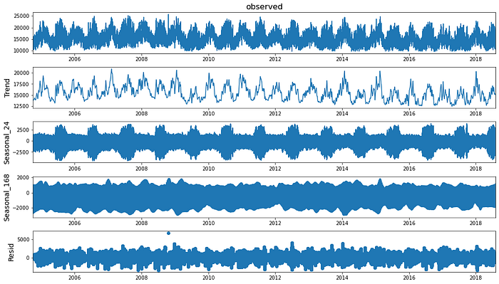
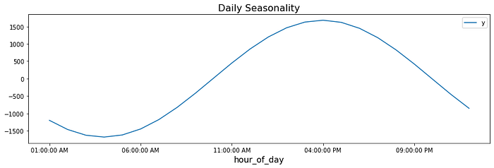
Generally, you would expect a daily pattern where energy consumption peaks during the day and declines at nighttime. Additionally, you would anticipate a weekly pattern where consumption is higher on weekdays compared to weekends when people travel or go outside more. An annual pattern is also expected, with higher energy consumption peaking in the summer than in other cooler months.

Daily pattern 3 days of January compared to July

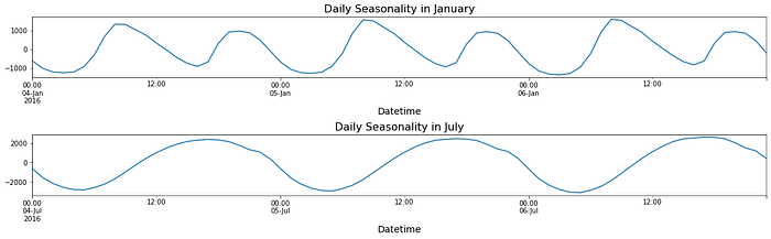
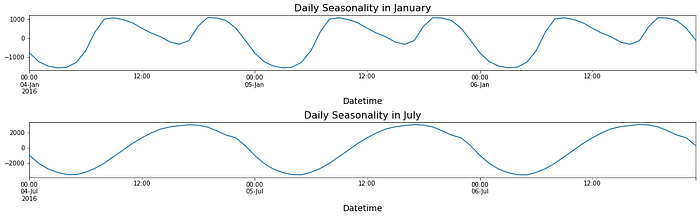
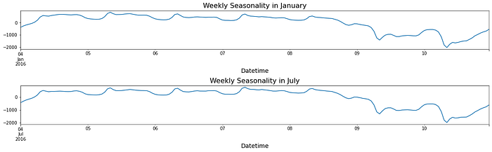
There is a repeating pattern of peaks during the day, which declines as it gets closer to the evening. Note that in the summertime, the daily pattern changes. For example, a daily pattern is similar in July, except the peak during the day is extended longer into later in the evening, possibly due to air conditoners being used at night before the weather cools down a little. Perform a similar slice for the weekly seasonal pattern:

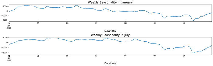
Overall, the results (from daily and weekly) suggest an annual influence indicative of an annual seasonal pattern. In the There’s more section, you will explore how you can expose this annual pattern (to capture repeating patterns every July as an example).

MSTL is a simple and intuitive algorithm for decomposing time series data with multiple seasonal patterns. The parameter iterate in MSTL defaults to iterate=2, which is the number of iterations the algorithm uses to estimate the seasonal components. At each iteration, the algorithm applies the STL algorithm to estimate the seasonal component for each seasonal period identified.

You will update windows to [121, 121] for each seasonal component in the following code. The default values for windows are [11, 15]. The default value for iterate is 2, and you will update it to 5.

mstl = MSTL(df, periods=(24, 24*7), iterate=4, windows=[121, 121])
results = mstl.fit()

You can use the same code from the previous section to plot the daily and weekly components. You will notice that the output is smoother due to the windows parameter (increased). The windows parameter accepts integer values to represent the length of the seasonal smoothers for each component. The values must be odd integers. The iterate determines the number of iterations to improve on the seasonal components. code here

Forecasting with multiple seasonal patterns using the Unobserved Components Model (UCM)

In the previous recipe, you were introduced to MSTL to decompose a time series with multiple seasonality. Similarly, the Unobserved Components Model (UCM) is a technique that decomposes a time series (with multiple seasonal patterns), but unlike MSTL, the UCM is also a forecasting model. Initially, the UCM was proposed as an alternative to the ARIMA model and introduced by Harvey in the book Forecasting, structural time series models and the Kalman filter, first published in 1989. Unlike an ARIMA model, the UCM decomposes a time series process by estimating its components and does not make assumptions regarding stationarity or distribution.

There are situations where making a time series stationary — for example, through differencing is not achievable. The time series can also contain irregularities and other complexities. This is where the UCM comes in as a more flexible and interpretable model. The UCM is based on the idea of latent variables or unobserved components of a time series, such as level, trend, and seasonality. These can be estimated from the observed variable. In statsmodels , the UnobservedComponents class decomposes a time series into a trend component, a seasonal component, a cyclical component, and an irregular component or error term. The equation can be generalized as the following:

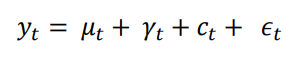
here, 𝑦𝑡 is the observed variable at time t, and 𝑢𝑡, 𝛾𝑡, 𝑐𝑡 represent the trend, seasonal, and cyclical components. The 𝜖𝑡 term is the irregular component (or disturbance). You can have multiple seasons as well. The main idea in the UCM is that each component, called state, is modeled in a probabilistic manner since they are unobserved. The UCM can also contain autoregressive and regression components to capture their effects.

In this recipe, you will use the UCM implementation in statsmodels. You will use the same energy dataset loaded in the Technical requirements section. In the Decomposing time series with multiple seasonal patterns using MSTL recipe, you were able to decompose the seasonal pattern into daily, weekly, and yearly components. You will use this knowledge in this recipe:

from statsmodels.tsa.statespace.structural import UnobservedComponents

UnobservedComponents take several parameters. Of interest is freq_seasonal, which takes a dictionary for each frequency-domain seasonal component — for example, daily, weekly, and annually. You will pass a list of key-value pairs for each period. Optionally, within each dictionary, you can also pass a key-value pair for harmonics. If no harmonic values are passed, then the default would be the np.floor(period/2)

params = {'level':'dtrend',  'irregular':True,  
         'freq_seasonal':[{'period': day},{'period': week},
         {'period': year}],  
         'stochastic_freq_seasonal':[False, False, False]} 
model = UnobservedComponents(train, **params)

You can now fit the model on the training data using the fit method and Once training is complete, you can view the model’s summary using the summary method

results = model.fit()
results.summary()

The results objects are of type UnobservedComponentsResultsWrapper, which gives access to several properties and methods, such as plot_components and plot_diagnostics, to name a few. plot_diagnostics is used to diagnose the model’s overall performance against the residuals:

Plotting the daily seasonal component

Plotting the weekly seasonal component

Plotting the yearly seasonal component

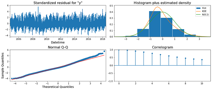
We had a similar observation in the previous recipe using MSTL

Finally, use the model to make a prediction and compare it against the out-of-sample set (test data) and Calculate the RMSE and RMSPE using the functions imported from statsmodels earlier in the Technical requirements section.
code here

rmspe(test['y'], prediction) 
>> 1.0676342700345198 
rmse(test['y'], prediction) 
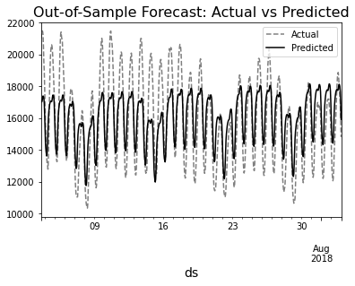
>> 1716.1196099493693

Forecasting time series with multiple seasonal patterns using Prophet

The goal of this recipe is to show how you can use Prophet to solve a more complex dataset with multiple seasonal patterns.

One benefit of using algorithms such as the UCM (introduced in the previous recipe) or Prophet is that they require little to no data preparation, can work with noisy data, and are easy to interpret. Another advantage is their ability to decompose a time series into its components (trend and multiple seasonal components)

In this recipe, you will continue using the same energy consumption dataset (the df DataFrame) and perform a similar split for the train and test sets

from prophet import Prophet 
from prophet.plot import add_changepoints_to_plot
energy = df.copy() 
energy.reset_index(inplace=True) 
energy.columns = ['ds', 'y']
train = energy.iloc[:-month] 
test = energy.iloc[-month:]
model = Prophet().fit(train)

Use the make_future_dataframe method to extend the train DataFrame forward for a specific number of periods and at a specified frequency. In this case, it will be the number of test observations. The frequency is indicated as hourly with freq= ‘H’.

n = len(test) 
future = model.make_future_dataframe(n, freq='H')
forecast = model.predict(future)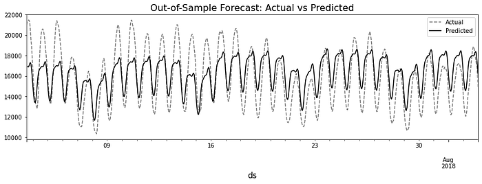

rmspe(test['y'].values, prediction.values) 
>> 1.2587190915113151 
rmse(test['y'].values, prediction.values) 
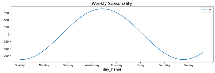
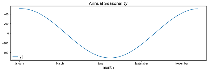
>> 1885.143242946697

Prophet automated many aspects of building and optimizing the model because yearly_ seasonality, weekly_seasonality, and daily_seasonality parameters were set to auto by default, allowing Prophet to determine which ones to turn on or off based on the data. So far, you have used Prophet on time series with single seasonality and now again on a time series with multiple seasonality. The process for training a model and making predictions is the same, making Prophet a very appealing option due to its consistent framework. code here

Forecasting time series with multiple seasonal patterns using NeuralProphet

NeuralProphet was inspired by the Prophet library and Autoregressive Neural Network (AR-Net) to bring a new implementation, leveraging deep neural networks to provide a more scalable solution.

Prophet was built on top of PyStan, a Bayesian inference library, and is one of the main dependencies when installing Prophet. Conversely, NeuralProphet is based on PyTorch and is as used as the deep learning framework. This allows NeuralProphet to scale to larger datasets & generally provides better accuracy than Prophet. Like Prophet method, NeuralProphet performs hyperparameter tuning and fully automates many aspects of time series forecasting. In this recipe, you will compare the results using NeuralProphet against Prophet.

You will use the same energy dataset created in the Forecasting time series with multiple seasonal patterns using Prophet recipe. Instead of splitting the dataset into train and test sets, you will split it into the train, validation, and test sets. The validation set will be used during the training process to evaluate at every epoch:

from neuralprophet import NeuralProphet
energy = df.copy() 
energy.reset_index(inplace=True) 
energy.columns = ['ds', 'y'] 
train = energy.iloc[:-month*2] 
val = energy.iloc[-month*2:-month] 
test = energy.iloc[-month:]
m = NeuralProphet() 
metrics = m.fit(train, validation_df=val)

Similar to Prophet, you will use the make_future_dataframe method to extend the train DataFrame forward for a specific number of periods & at a specified frequency. In this case, it will be the total number of test and val observations:

n = len(test)+len(val) 
future = m.make_future_dataframe(df=train, periods=n) 
forecast = m.predict(df=future)
fig = m.plot_components(forecast)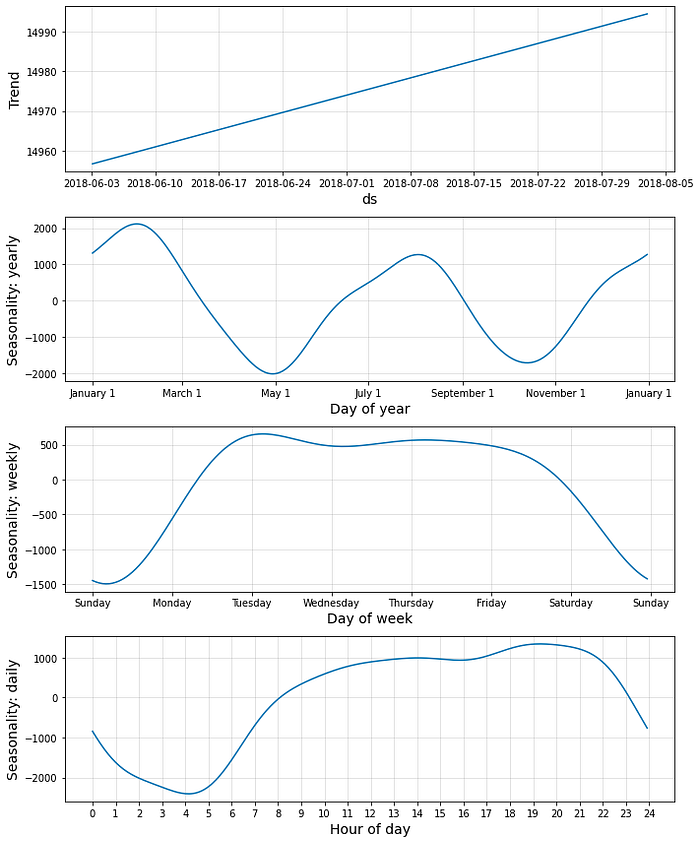

The time series seasonal components automatically detected by NeuralProphet

rmspe(test['y'].values, prediction.values) 
>> 1.1729025662066894 
rmse(test['y'].values, prediction.values) 
>> 1796.2832495706689

Overall, both RMSE and RMSPE for NeuralProphet indicate that the model outperforms Prophet

Similar to Prophet, NeuralProphet also decomposes a time series into its components. NeuralProphet can include different terms such as trend, seasonality, autoregression (the n_lags parameter), special events (the add_events method), future regressors (exogenous variables with the add_future_regressor method), and lagged regressors (the add_lagged_ regressor method). The autoregression piece is based on AR-Net, an auto- regressive neural network. NeuralProphet allows you to add recurring special events — for example, a Superbowl game or a birthday. The time series modeling process is similar to that in Prophet, which was made by design. Keep in mind that NeuralProphet was built from the ground up, leveraging PyTorch, and is not a wrapper to Prophet. code here