Outlier/Anomalies Detection Using Unsupervised Machine Learning
Outlier detection is not straightforward, mainly due to the ambiguity surrounding the definition of what an outlier is specific to your data or the problem that you are trying to solve.

The recipes that you will encounter in this chapter are as follows:
- Detecting outliers using KNN
- Detecting outliers using LOF
- Detecting outliers using iForest
- Detecting outliers using One-Class Support Vector Machine (OCSVM)
- Detecting outliers using COPOD
- Detecting outliers with PyCaret
Load the nyc_taxi.csv data into a pandas DataFrame and create plot_outliers function that you will use throughout the recipes
The preceding code should produce a time series plot with x markers for the known outliers:

PyOD is one such library to detect outliers in your data. It provides access to more than 20 different algorithms to detect outliers and is compatible with both Python 2 and 3. An absolute gem!
Detecting outliers using KNN
In the case of outlier detection, the algorithm is used differently. Since we do not know the outliers in advance, KNN is used in an unsupervised learning manner. In this scenario, the algorithm finds the closest K nearest neighbors for every data point and measures the average distance. The points with the most significant distance from the population will be considered outliers, and more specifically, they are considered global outliers. hence KNN is a proximity-based algorithm.
Generally, proximity-based algorithms rely on the distance or proximity between an outlier point and its nearest neighbors. In KNN, the number of nearest neighbors, k, is a parameter you need to determine. There are other variants of the KNN algorithm supported by PyOD, for example, Average KNN (AvgKNN), which uses the average distance to the KNN for scoring, and Median KNN (MedKNN), which uses the median distance for scoring.
Start by loading the KNN class:
from pyod.models.knn import KNNBefore going further you should be familiar with a few parameters to control the algorithm’s behavior. The first parameter is contamination, which is a common parameter across all the different classes (algorithms) in PyOD. For example, a contamination value of 0.1 indicates that you expect 10% of the data to be outliers. The default value is contamination=0.1. The value for contamination range from 0 to 0.5 (or 50%).
The second parameter, specific to KNN, is a method, which defaults to method=‘largest ’. In this recipe, you will change it to the mean (the average of all k neighbor distances). The third parameter, also specific to KNN, is a metric, which tells the algorithm how to compute the distances. The default is the minkowski distance but it can take any distance metrics from scikit-learn or the SciPy library. Finally, you need to provide the number of neighbors, which defaults to n_neighbors=5. Ideally, you will want to run for different KNN models with varying values of k and compare the results to determine the optimal number of neighbors. You will need to experiment with these parameters.
Instantiate KNN with the updated parameters and then train (fit) the model:
knn = KNN(contamination=0.03,method='mean',n_neighbors=5) knn.fit(tx)The predict method will generate binary labels, either 1 or 0, for each data point. A value of 1 indicates an outlier. Store the results in a pandas Series and filter the predicted Series to only show the outlier values
predicted = pd.Series(knn.predict(tx),index=tx.index)
print('Number of outliers = ', predicted.sum())
Overall, the results look promising; four out of the five known dates have been identified. Additionally, the algorithm identified the day after Christmas as well as January 26, 2015, which was when all vehicles were ordered off the street due to the North American blizzard
Use the plot_outliers function created in the Technical requirements section to visualize the output to gain better insight:

The unsupervised approach to the KNN algorithm calculates the distance of observation to other neighboring observations. The default distance used in PyOD for KNN is the Minkowski distance (the p-norm distance). You can change to different distance measures, such as the Euclidean distance with euclidean or l2 or the Manhattan distance with manhattan or l1.
Traditionally, when people hear KNN, they immediately assume it is only a supervised learning algorithm. For unsupervised KNN, there are three popular algorithms: ball tree, KD tree, and brute-force search. The PyOD library supports all three as ball_tree, kd_ tree, and brute, respectively. The default value is set to algorithm=‘auto’.
PyOD uses an internal score specific to each algorithm, scoring each observation in the training set. The decision_scores_ attribute will show these scores for each observation. Higher scores indicate a higher potential of being an abnormal observation and you can convert this into a DataFrame:
knn_scores = knn.decision_scores_
knn_scores_df = (pd.DataFrame(scores,index=tx.index,
                                           columns='score']))
knn_scores_df
Since all the data points are scored, PyOD will determine a threshold to limit the number of outliers returned. The threshold value depends on the contamination value you provided earlier (the proportion of outliers you suspect). The higher the contamination value, the lower the threshold, and hence more outliers are returned. A lower contamination value will increase the threshold. You can get the threshold value using the threshold_ attribute from the model after fitting it to the training data. Here is the threshold for KNN based on a 3% contamination rate:
knn.threshold_
>> 225.0179166666657
This is the value used to filter out the significant outliers. Here is an example of how you reproduce that:
knn_scores_df[knn_scores_df['score'] >= knn.threshold_].sort_
                                  values('score', ascending=False)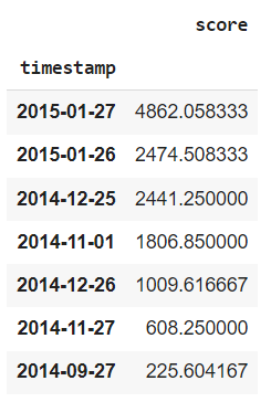
Notice the last observation on 2014–09–27 is slightly above the threshold, but it was not returned when you used the predict method. If you use the contamination threshold, you can get a better cutoff:
n = int(len(tx)*0.03)
knn_scores_df.nlargest(n, 'score')
Another helpful method is predict_proba, which returns the probability of being normal and the probability of being abnormal for each observation. PyOD provides two methods for determining these percentages: linear or unify. For ex., in the case of linear, the implementation uses MinMaxScaler from scikit-learn to scale the scores before calculating the probabilities. The unify method uses the z-score (standardization) and the Gaussian error function (erf) from the SciPy library (scipy.special.erf).
knn_proba = knn.predict_proba(tx, method='linear')
knn_proba_df = (pd.DataFrame(np.round(knn_proba * 100, 3),
                    index=tx.index,columns=['Proba_Normal',
                                           'Proba_Anomaly']))
knn_proba_df.nlargest(n, 'Proba_Anomaly')
For the unify method, you can just update method=‘unify’.
Detecting outliers using LOF
A data point far from its KNN can be considered an outlier. Overall, the algorithm does a good job of capturing global outliers, but those far from the surrounding points may not do well with identifying local outliers. This is where the LOF comes in to solve this limitation
Instead of using the distance between neighboring points, it uses density as a basis for scoring data points and detecting outliers. The LOF is considered a density-based algorithm. The idea behind the LOF is that outliers will be further from other data points and more isolated, and thus will be in low-density regions.
It is easier to illustrate this with an example: imagine a person standing in line in a small but busy Starbucks, and everyone is pretty much close to each other; then, we can say the person is in a high-density area and, more specifically, high local density. If the person decides to wait in their car in the parking lot until the line eases up, they are isolated and in a low-density area, thus being considered an outlier. From the perspective of the people standing in line, who are probably not aware of the person in the car, that person is considered not reachable even though that person in the vehicle can see all of the individuals standing in line. So we say that the person in the car is not reachable from their perspective. Hence, we sometimes refer to this as inverse reachability (how far you are from the neighbors’ perspective, not just yours).
Like KNN, you still need to define the k parameter for the number of nearest neighbors. The nearest neighbors are identified based on the distance measured between the observations (think KNN), then Local Reachability Density (LRD or local density for short) is measured for each neighboring point. This local density is the score used to compare the kth neighboring observations and those with lower local densities than their kth neighbors are considered outliers (they are further from the reach of their neighbors).
Start by loading the LOF class:
from pyod.models.lof import LOFInstantiate LOF by updating n_neighbors=5 and contamination=0.03 while keeping the rest of the parameters with the default values. Then, train (fit) the model:
lof = LOF(contamination=0.03, n_neighbors=5)
lof.fit(tx)
The predict method will output either 1 or 0 for each data point. A value of 1 indicates an outlier. Store the results in a pandas Series & filter the predicted Series to only show the outlier values:
predicted = pd.Series(lof.predict(tx),index=tx.index)
print('Number of outliers = ', predicted.sum())
outliers = predicted[predicted == 1]
outliers = tx.loc[outliers.index]
outliers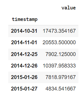
Interestingly, it captured three out of the five known dates but managed to identify the day after Thanksgiving and the day after Christmas as outliers. Additionally, October 31 was on a Friday, and it was Halloween night.

LOF is like KNN in that we measure the distances between the neighbors before calculating the local density. The local density is the basis of the decision scores, which you can view using the decision_scores_ attribute:
timestamp   score
2014-11-01  14.254309
2015-01-27  5.270860
2015-01-26  3.988552
2014-12-25  3.952827
2014-12-26  2.295987
2014-10-31  2.158571
The scores are very different from KNN
Like the LOF, another extension of the algorithm is the Cluster-Based Local Outlier Factor (CBLOF). The CBLOF is similar to LOF in concept as it relies on cluster size and distance when calculating the scores to determine outliers. So, instead of the number of neighbors (n_neighbors like in LOF), we now have a new parameter, which is the number of clusters (n_clusters). The default clustering estimator, clustering_estimator, in PyOD is the k-means clustering algorithm.
from pyod.models.cblof import CBLOF
cblof = CBLOF(n_clusters=4, contamination=0.03)
cblof.fit(tx)
predicted = pd.Series(lof.predict(tx),index=tx.index)
outliers = predicted[predicted == 1]
outliers = tx.loc[outliers.index]
plot_outliers(outliers, tx, 'CBLOF')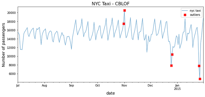
Compare the above figure with (LOF) figure and notice the similarity.
Detecting outliers using iForest
iForest has similarities with another popular algorithm known as Random Forests. iForest, also an ensemble learning method, is the unsupervised learning approach to Random Forests. The iForest algorithm isolates anomalies by randomly partitioning (splitting) a dataset into multiple partitions. This is performed recursively until all data points belong to a partition. The number of partitions required to isolate an anomaly is typically smaller than the number of partitions needed to isolate a regular point. The idea is that an anomaly data point is further from other points and thus easier to separate (isolate).
In contrast, a normal data point is probably clustered closer to the larger set and, therefore, will require more partitions (splits) to isolate that point. Hence the name, isolation forest, since it identifies outliers through isolation. Once all the points are isolated, the algorithm will create an outlier score. You can think of these splits as creating a decision tree path. The shorter the path length to a point, the higher the chances of an anomaly.
Start by loading the IForest class:
from pyod.models.iforest import IForestInstantiate IForest and update the contamination &random_state parameters. Then, fit the new instance of the class (iforest) on the resampled data to train the model:
iforest = IForest(contamination=0.03,n_estimators=100,
                                             random_state=0)
iforest.fit(nyc_daily)
predicted = pd.Series(iforest.predict(tx),index=tx.index)
print('Number of outliers = ', predicted.sum())
>> Number of outliers =  7
outliers = predicted[predicted == 1]
outliers = tx.loc[outliers.index]
outliers
>>  timestamp   value
    2014-11-01  20553.500000
    2014-11-08  18857.333333
    2014-11-27  10899.666667
    2014-12-25  7902.125000
    2014-12-26  10397.958333
    2015-01-26  7818.979167
    2015-01-27  4834.541667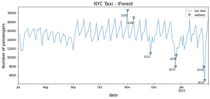
Detecting outliers using One-Class Support Vector Machine (OCSVM)
In addition to classification and regression, Support Vector Machine (SVM) can also be used for outlier detection in an unsupervised manner, similar to KNN, which is mostly known as a supervised machine learning technique but was used in an unsupervised manner for outlier detection, as seen in the Outlier detection using KNN recipe.
Start by loading the OCSVM class:
from pyod.models.ocsvm import OCSVM
ocsvm = OCSVM(contamination=0.03, kernel='rbf')
ocsvm.fit(tx)
predicted = pd.Series(ocsvm.predict(tx),index=tx.index)
print('Number of outliers = ', predicted.sum())
>>  Number of outliers =  5outliers = predicted[predicted == 1]
outliers = tx.loc[outliers.index]
outliers
>>  timestamp   value
    2014-08-09  15499.708333
    2014-11-18  15499.437500
    2014-11-27  10899.666667
    2014-12-24  12502.000000
    2015-01-05  12502.750000
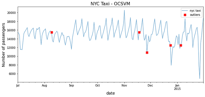
When examining the plot, it is not clear why OCSVM picked up on those dates as being outliers. The RBF kernel can capture non-linear relationships, so you would expect it to be a robust kernel. The reason for this inaccuracy is that SVM is sensitive to data scaling. To get better results, you will need to standardize (scale) your data first.
from pyod.utils.utility import standardizer
scaled = standardizer(tx)
predicted = pd.Series(ocsvm.fit_predict(scaled),index=tx.index)
outliers = predicted[predicted == 1]
outliers = tx.loc[outliers.index]
outliers
>>  timestamp   value
    2014-07-06  11464.270833
    2014-11-01  20553.500000
    2014-11-27  10899.666667
    2014-12-25  7902.125000
    2014-12-26  10397.958333
    2015-01-26  7818.979167
    2015-01-27  4834.541667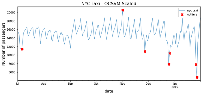
Compare the results from the before fig and after fig to see how scaling made a big difference in how the OCSVM algorithm identified outliers
You can explore how the different kernels ‘linear’, ‘poly’, ‘rbf’, and ‘sigmoid’ perform on the same dataset
Detecting Outliers using Copula-Based Outlier Detection (COPOD)
COPOD is an exciting algorithm based on a paper published in September 2020, which you can read here
The PyOD library offers many algorithms based on the latest research papers, which can be broken down into linear models, proximity-based models, probabilistic models, ensembles, and neural networks.
COPOD falls under probabilistic models and is inspired by statistical methods, making it a fast and highly interpretable model. The algorithm is based on copula, a function generally used to model dependence between independent random variables that are not necessarily normally distributed. In time series forecasting, copulas have been used in univariate and multivariate forecasting, which is popular in financial risk modeling. The term copula stems from the copula function joining (coupling) univariate marginal distributions to form a uniform multivariate distribution function.
Start by loading the COPOD class:
from pyod.models.copod import COPOD
copod = COPOD(contamination=0.03)
copod.fit(tx)
predicted = pd.Series(copod.predict(tx),index=tx.index)
print('Number of outliers = ', predicted.sum())
>>  Number of outliers =  7
outliers = predicted[predicted == 1]
outliers = tx.loc[outliers.index]
outliers
>>  timestamp   value
    2014-07-04  11511.770833
    2014-07-06  11464.270833
    2014-11-27  10899.666667
    2014-12-25  7902.125000
    2014-12-26  10397.958333
    2015-01-26  7818.979167
    2015-01-27  4834.541667
For more insight into decision_scores_, threshold_, or predict_proba, please review the first recipe Detecting outliers using KNN. code here
Detecting outliers with PyCaret
In this recipe, you will explore PyCaret for outlier detection. PyCaret is positioned as “an open-source, low-code machine learning library in Python that automates machine learning workflows”. It acts as a wrapper for PyOD, which you used earlier in the previous recipes for outlier detection. What PyCaret does is simplify the entire process for rapid prototyping and testing with a minimal amount of code. You will use PyCaret to examine multiple outlier detection algorithms, similar to the ones you used in earlier recipes, and see how PyCaret simplifies the process for you.
Start by loading all the available functions from the pycaret.anomaly module:
from pycaret.anomaly import *
setup = setup(tx, session_id = 1, normalize=True)
To print a list of available outlier detection algorithms, you can run models():
models()Notice these are all sourced from the PyOD library. As stated earlier, PyCaret is a wrapper on top of PyOD and other libraries, such as scikit-learn.
Let’s store the names of the first eight algorithms in a list to use later:
list_of_models = models().index.tolist()[0:8]
list_of_models
>>
     ['abod', 'cluster', 'cof', 'iforest', 'histogram', 'knn', 'lof', 'svm']
Loop through the list of algorithms and store the output in a dictionary so you can reference it later for your analysis. To create a model in PyCaret, you simply use the create_model() function. This is similar to the fit() function in scikit-learn and PyOD for training the model. Once the model is created, you can use the model to predict (identify) the outliers using the predict_model() function. PyCaret will produce a DataFrame with three columns: the original value column, a new column, Anomaly, which stores the outcome as either 0 or 1, where 1 indicates an outlier, and another new column, Anomaly_Score, which stores the score used (the higher the score, the higher the chance it is an anomaly).
You will only change the contamination parameter to match earlier recipes using PyOD. In PyCaret, the contamination parameter is called fraction, and to be consistent, you will set that to 0.03 or 3% with fraction=0.03:
results = {}
for model in list_of_models:
    cols = ['value', 'Anomaly_Score']
    outlier_model = create_model(model, fraction=0.03)
    print(outlier_model)
    outliers = predict_model(outlier_model, data=tx)
    outliers = outliers[outliers['Anomaly'] == 1][cols]
    outliers.sort_values('Anomaly_Score', ascending=False,
                                                inplace=True)
    results[model] = {'data': outliers, 'model': outlier_ model}
The results dictionary contains the output (a DataFrame) from each model.
PyCaret is a great library for automated machine learning, and recently they have been expanding their capabilities around time series analysis and forecasting and anomaly (outlier) detection. PyCaret is a wrapper over PyOD, the same library you used in earlier recipes of this article. code here